
Who Scores the Most Expensive Basket in the NBA?
Hey! Just a quick post after work. A couple weeks ago, my roommate showed me a tweet that listed soccer players with the most expensive contracts. (I think it was the Premier League?) Of course, I wanted to make something similar with NBA players. I made some quick bar graphs that night showing $ earned per made basket, which was cool, but I wanted to make it a little better.
In this post, I’m going to a good old bar graph. Let’s dive in to this!
I have three dataframes that I pulled from the nbastatR package.
library(tidyverse)

df_salary <- read_csv("salary2020.csv")
df_salary
## # A tibble: 523 x 2
## namePlayer amountContract
## <chr> <dbl>
## 1 Otto Porter 27250576
## 2 Zach LaVine 19500000
## 3 Thaddeus Young 12900000
## 4 Tomas Satoransky 10000000
## 5 Cristiano Felicio 8156500
## 6 Kris Dunn 5348007
## 7 Coby White 5307120
## 8 Lauri Markkanen 5300400
## 9 Wendell Carter 5201400
## 10 Denzel Valentine 3377568
## # ... with 513 more rowsdf_stats <- read_csv("all2020.csv") %>%
select(namePlayer, slugTeam, fgm)
df_stats## # A tibble: 505 x 3
## namePlayer slugTeam fgm
## <chr> <chr> <dbl>
## 1 Aaron Gordon ORL 253
## 2 Aaron Holiday IND 181
## 3 Abdel Nader OKC 73
## 4 Adam Mokoka CHI 6
## 5 Admiral Schofield WAS 30
## 6 Al Horford PHI 241
## 7 Al-Farouq Aminu ORL 25
## 8 Alec Burks PHI 244
## 9 Alen Smailagic GSW 19
## 10 Alex Caruso LAL 90
## # ... with 495 more rowsphotos <- read_csv("photos.csv") %>%
select(namePlayer, urlPlayerHeadshot)
photos## # A tibble: 4,506 x 2
## namePlayer urlPlayerHeadshot
## <chr> <chr>
## 1 Alaa Abdelnaby https://ak-static.cms.nba.com/wp-content/uploads/headshots~
## 2 Zaid Abdul-Aziz https://ak-static.cms.nba.com/wp-content/uploads/headshots~
## 3 Kareem Abdul-Jab~ https://ak-static.cms.nba.com/wp-content/uploads/headshots~
## 4 Mahmoud Abdul-Ra~ https://ak-static.cms.nba.com/wp-content/uploads/headshots~
## 5 Tariq Abdul-Wahad https://ak-static.cms.nba.com/wp-content/uploads/headshots~
## 6 Shareef Abdur-Ra~ https://ak-static.cms.nba.com/wp-content/uploads/headshots~
## 7 Tom Abernethy https://ak-static.cms.nba.com/wp-content/uploads/headshots~
## 8 Forest Able https://ak-static.cms.nba.com/wp-content/uploads/headshots~
## 9 John Abramovic https://ak-static.cms.nba.com/wp-content/uploads/headshots~
## 10 Alex Abrines https://ak-static.cms.nba.com/wp-content/uploads/headshots~
## # ... with 4,496 more rowsNow that I’ve extracted the info I’m interested in, (field goal made and player photos) Let’s join them into a single dataframe.
salaried_stats <- df_stats %>%
  inner_join(df_salary, by = "namePlayer") %>%
  inner_join(photos, by = "namePlayer")
salaried_stats
## # A tibble: 425 x 5
## namePlayer slugTeam fgm amountContract urlPlayerHeadshot
## <chr> <chr> <dbl> <dbl> <chr>
## 1 Aaron Gordon ORL 253 19863636 https://ak-static.cms.nba.com/wp~
## 2 Aaron Holiday IND 181 2239200 https://ak-static.cms.nba.com/wp~
## 3 Abdel Nader OKC 73 1618520 https://ak-static.cms.nba.com/wp~
## 4 Adam Mokoka CHI 6 79568 https://ak-static.cms.nba.com/wp~
## 5 Admiral Scho~ WAS 30 1000000 https://ak-static.cms.nba.com/wp~
## 6 Al Horford PHI 241 28000000 https://ak-static.cms.nba.com/wp~
## 7 Al-Farouq Am~ ORL 25 9258000 https://ak-static.cms.nba.com/wp~
## 8 Alec Burks PHI 244 2320044 https://ak-static.cms.nba.com/wp~
## 9 Alen Smailag~ GSW 19 898310 https://ak-static.cms.nba.com/wp~
## 10 Alex Caruso LAL 90 2750000 https://ak-static.cms.nba.com/wp~
## # ... with 415 more rowsMaking the graphs
Since many players don’t get to play in the NBA, I’ve filtered for only players that scored at least 100 baskets. Then, I can calculate the $ made per basket.
per_bucket <- salaried_stats %>%
  mutate(money_per_buckets = amountContract / fgm) %>%
  filter(fgm >= 100)
per_bucket
## # A tibble: 211 x 6
## namePlayer slugTeam fgm amountContract urlPlayerHeadshot money_per_bucke~
## <chr> <chr> <dbl> <dbl> <chr> <dbl>
## 1 Aaron Gord~ ORL 253 19863636 https://ak-static~ 78512.
## 2 Aaron Holi~ IND 181 2239200 https://ak-static~ 12371.
## 3 Al Horford PHI 241 28000000 https://ak-static~ 116183.
## 4 Alec Burks PHI 244 2320044 https://ak-static~ 9508.
## 5 Alex Len SAC 142 4160000 https://ak-static~ 29296.
## 6 Andre Drum~ CLE 367 27093018 https://ak-static~ 73823.
## 7 Andrew Wig~ GSW 365 27504630 https://ak-static~ 75355.
## 8 Anfernee S~ POR 178 2149560 https://ak-static~ 12076.
## 9 Anthony Da~ LAL 416 27093019 https://ak-static~ 65127.
## 10 Aron Baynes PHX 146 5453280 https://ak-static~ 37351.
## # ... with 201 more rowsI wonder what the league-wide average was?
library(scales)
avg_bucket_pay <- as.numeric(per_bucket %>% summarize(mean(money_per_buckets)))
dollar(avg_bucket_pay)
## [1] "$48,838.41"That’s a lot of money! If you make a basket in the NBA, you’re pretty much making as much as a regular Joe will make in an entire year!
Most expensive baskets
I arranged the dataframe in a descending order of $ per basket, took top 10, and made a bar graph with geom_col. After that, I used geom_image from ggimage package to plot a player’s headshot at the end of the bar graphs.
library(ggimage)
theme_set(theme_light())

per_bucket %>%
  arrange(desc(money_per_buckets)) %>%
  slice(1:10) %>%
  mutate(namePlayer = fct_reorder(namePlayer, money_per_buckets)) %>%
  ggplot(aes(namePlayer, money_per_buckets, fill = fgm)) +
  geom_col() +
  geom_image(aes(image = urlPlayerHeadshot), size = 0.1) +
  geom_hline(yintercept = avg_bucket_pay, linetype = "dashed") +
  geom_text(aes(3, avg_bucket_pay, label = "League Avg. $48,838")) +
  coord_flip() +
  scale_fill_gradient2(low = "blue", mid = "pink", high = "red", midpoint = 200) +
  scale_y_continuous(labels = dollar_format()) +
  labs( title = "Who scores the most expensive buckets in 2020 NBA season?",
        subtitle = "At least 100 Fg Made this season",
        x = "",
        y = "$ per field goal made",
fill = "# made field goal") 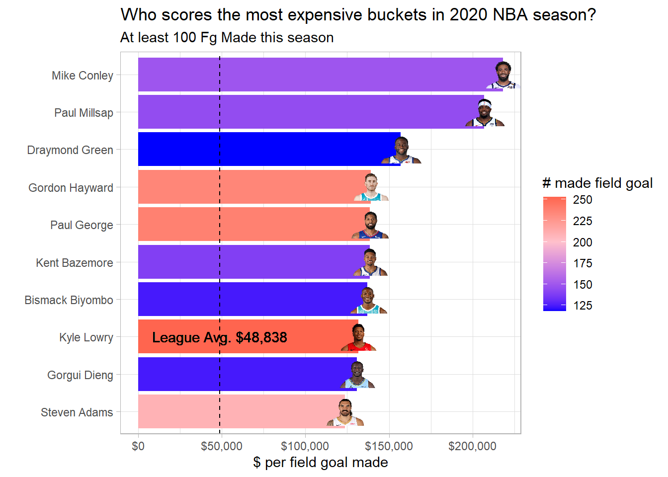
Don’t really see too obvious a pattern. Some of them are defense-first guys (Green, Bazemore & Biyombo), while some are legit scorers (Hayward, George & Lowry). Now, let’s look at the most economically friendly contracts.
The Cheapest baskets
This is basically the same plot as above, but I took the ascending order of $ per basket instead.
per_bucket %>%
  arrange((money_per_buckets)) %>%
  slice(1:10) %>%
  mutate(namePlayer = fct_reorder(namePlayer, -money_per_buckets)) %>%
  ggplot(aes(namePlayer, money_per_buckets, fill = fgm)) +
  geom_col() +
  geom_image(aes(image = urlPlayerHeadshot), size = 0.1) +
  geom_hline(yintercept = avg_bucket_pay, linetype = "dashed") +
  geom_text(aes(3, 30000, label = "League Avg. $48,838")) +
  coord_flip() +
  scale_fill_gradient2(low = "blue", mid = "pink", high = "red", midpoint = 200) +
  scale_y_continuous(labels = dollar_format()) +
  labs( title = "Who scores the most economical buckets in 2020 NBA season?",
                subtitle = "At least 100 Fg Made this season",
  x = "",
  y = "$ per field goal made",
fill = "# made field goal") 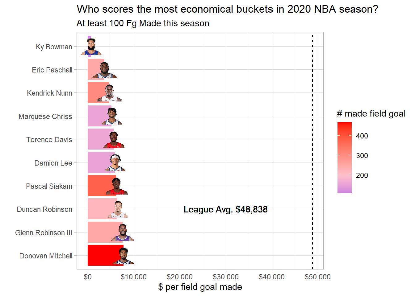
Obvious pattern is the youth of this group of players. All of these guys are in their early-mid 20s, who are under their rookie contracts. We see Toronto’s Pascal Siakam & Terrance Davis in the mix, which is nice to see from a Raps fan. Furthermore, there are 4 Golden State Warriors (5 if you count Glenn Robinson who got traded this month). This makes sense, as Golden State’s stars have been injured all season, forcing them to play their inexperienced players.
Ky Bowman
You may have noticed Ky Bowman’s ubsurdly low $ per basket. He was on a 45-day 2-way contract, which means he can go back and forth between an NBA team and a farm team. His salary is less than $80,000, which I know some of you make more than! Unfortunately for him, he plays in the city of San Francisco, which is notorious for its expensive rent. There was a rumor that he may qualify for a low income housing, which turned out not to be true. However, due to his performance as of late, the Warrios signed him to a multi-year contract
Conclusion
I had a super fun time writing this post, and learned a couple of new tricks. One thing I could do next time, is to investigate if there is a relationship between the number of efficient contracts to team performance. Maybe I can count the number of players with below league average $ per basket, and use that as a variable to predict the number of wins.