Predicting CAD/USD Exchange Rate with K-nearest Neighbour Algorithm

What is K-nearest neighbour?

Below is a graph with two arbitrary classes: green squares and blue triangles. Our goal is to correctly predict whether a random new point (red circle) should be classified as a blue triangle or a green square. To do this, kNN identifies top k closest points. (in this case 3 in the red boundary) Of the 3, there are 2 blue triangles, and one green square. kNN then decides that the red circle must be a blue triangle based on chances. (66.66% vs 33.33%)

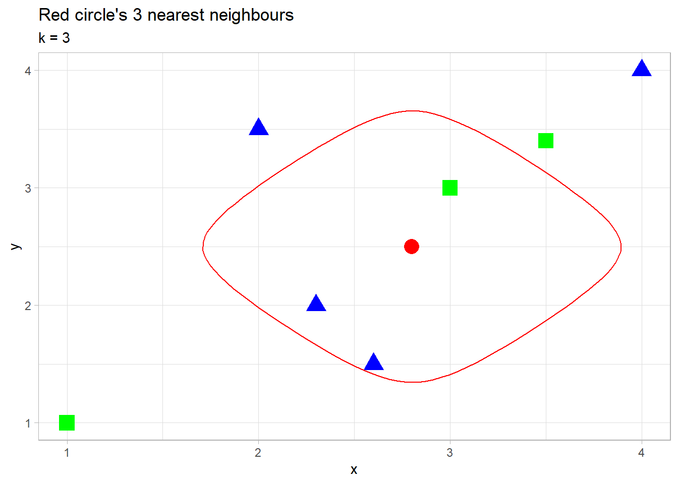
Figure 1: knn applied to a single point

This is the essential rationale behind the KNN algorithm. Despite its simplicity, it yields surprisingly robust results. In general, the steps in the k-Nearest Neighbour algorithm are:

1. Calculate the distance between all points and the point of interest (red circle)
2. Arrange by shortest distance and take top k of them
3. Find the most common class and assign it to the point of interest

kNN in Time Series

kNN can be applied to answer questions involving time such as

• “How many times have the raptors consecutively won the first 3 games in the season, and what typically happened in the 4th game?”
• “Last time it was -30 degrees in January, the temprature of the following months were a little better, would it be the same this year?”
• The technical analysis in finance. (buying stocks because of the movements in stock prices, rather than seeing the intrinsic value of the company)

What the above three all have in common is the recognition of patterns. Let’s say there were 8 years the raptors started the season 3-0. Then, each of those 3-game stretch is considered a neighbour to the current year’s 3-game winning streak from the opening night. Consequently, the outcome of the 4th game in each of those neighbours will be averaged to come to a conclusion that the raptors will most likely win.

Same thing in finance. Take for example, a trading strategy where you buy all stocks that lost more than 3% today, hoping it would go up tomorrow. Someone using this strategy must have considered every single instance in history where a stock lost more than 3% in one day, and came to a conclusion that on average, these stocks do well the next day. Of course, this type analysis is frowned upon in the finance field because of the efficient market hypothesis (EMH). In its core, the EMH teaches finance students that they can’t consistently beat the market no matter how good they are at finding good stocks, because the market already knows about those stocks. Therefore, buyers of these stocks are actually paying fair values, rather than the bargain they thought they were getting.

But I’m going to do it anyways. Using the tsfknn package, I attempted to predict the 2019 CAD/USD exchange rate. Since it took too long for my ancient Acer laptop to handle the volume of daily data, I used monthly 😅

Implementation in R

The objective is to predict the movement of the exchange rate graph in 2019, by using the information from Jan-Dec 2018. We do this by looking up other instances in history that had similar movements as 2018, and seeing what happened in the subsequent years.

Now, we load in the tsfknn package, as well as tidyverse and lubridate, which is for used for data wrangling.

library(tidyverse)
library(tsfknn)
library(lubridate)

Here’s the dataset. You can ignore the days on dates, as they were set to the last day of the month, not the last trading day.

exchange <- read_csv("exchange_rate.csv", col_types = cols())
exchange %>% head()

## # A tibble: 6 x 2
##   time        rate
##   <date>     <dbl>
## 1 1972-01-31 0.994
## 2 1972-02-28 0.999
## 3 1972-03-31 1.00 
## 4 1972-04-30 1.01 
## 5 1972-05-31 1.02 
## 6 1972-06-30 1.01

Timeseries object is created with the end date set to December 2018, so we can evaluate the predictions of the model against the real data so far in 2019.

exchange_ts <- ts(exchange$rate, start=c(1972,1), end=c(2018,12), frequency=12)

Before looking at the entire dataset, let’s see if the past decade had any other similar patterns that CAD/USD experienced in 2018.

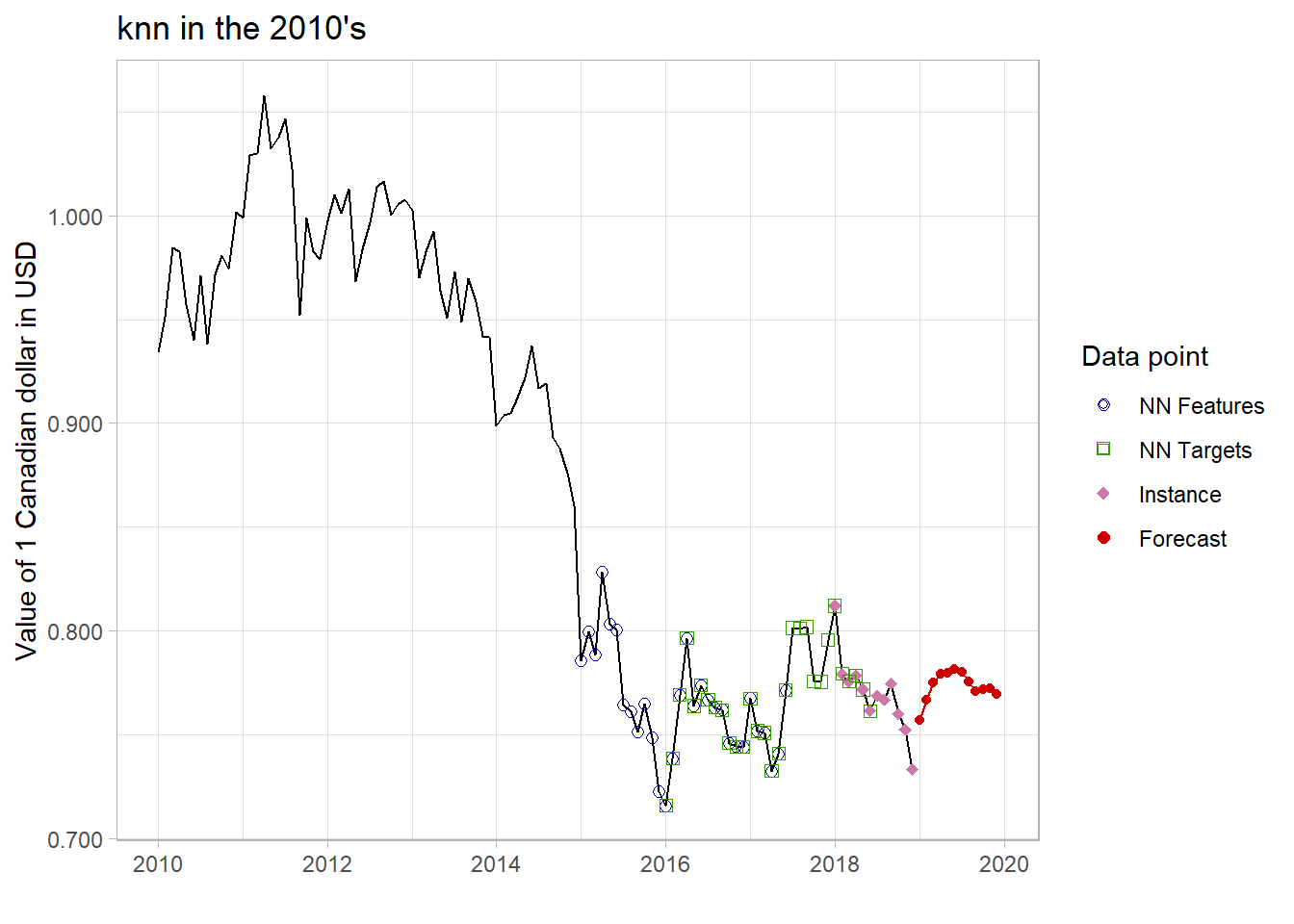
Figure 2: kNN captured 2 neighbours

Instance, the pink diamonds, is the pattern to be searched. Blue represents the neighbours, and Green represents what happened to these neighbours 12 months after the pattern. We then average the subsequent movements of the exchange rates of each neighbour (green) to predict CAD/USD for the 12 months in 2019, which is represented by red dots.

Based on the past decade, the 2019 looks to be a great year for the Canadian dollar. Now, let’s look at the entire dataset. Firstly, we take the trailing 12-months from Dec 2018, (lags = 1:12) and identify 100 other periods (k = 100) in the time frame where the patterns were similar. Then, calculate the mean movement of those patterns for the subsequent 12 months. (h = 12) Using these information, the knn_forecasting function applies kNN regression to a time series, and returns the predictions.

pred <- knn_forecasting(exchange_ts, h = 12, lags = 1:12, k = 100)

autoplot(pred, highlight = "neighbors", faceting = FALSE) +
  scale_y_continuous(labels = scales::number_format(accuracy = 0.001,
                                            decimal.mark = '.')) +
  labs(title =  "Canadian/US dollar exchange rate 1970-2019",
       x = "",
       y = "Value of 1 Canadian dollar in USD")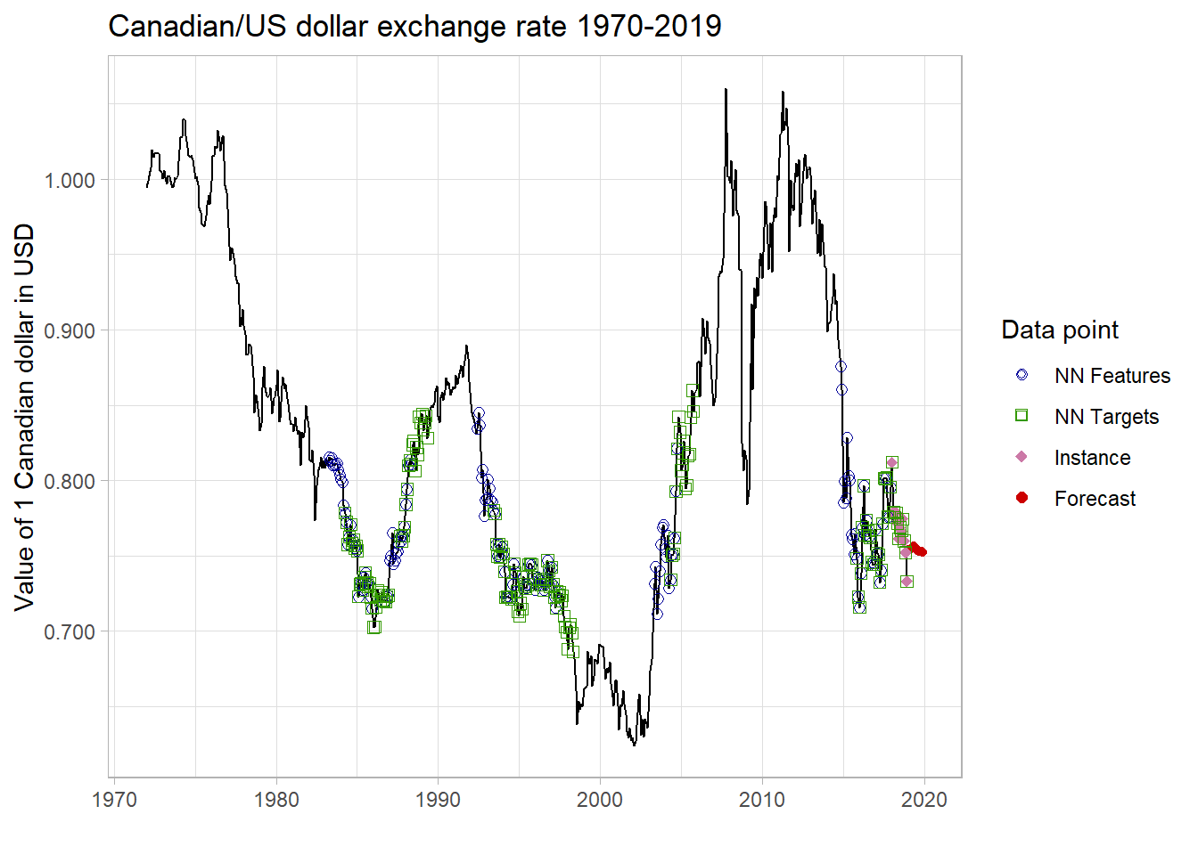

Figure 3: Lots of neighbours from the mid 80’s and the mid 90’s

Prediction

The red line is my prediction with kNN. As you can see, it’s dead wrong. I predicted the rate to stay at the similar level without much volatility, but the actual data from January to July was quite different. Although my model somewhat predicted the most recent rate, it failed to capture the ups and downs in 2019.

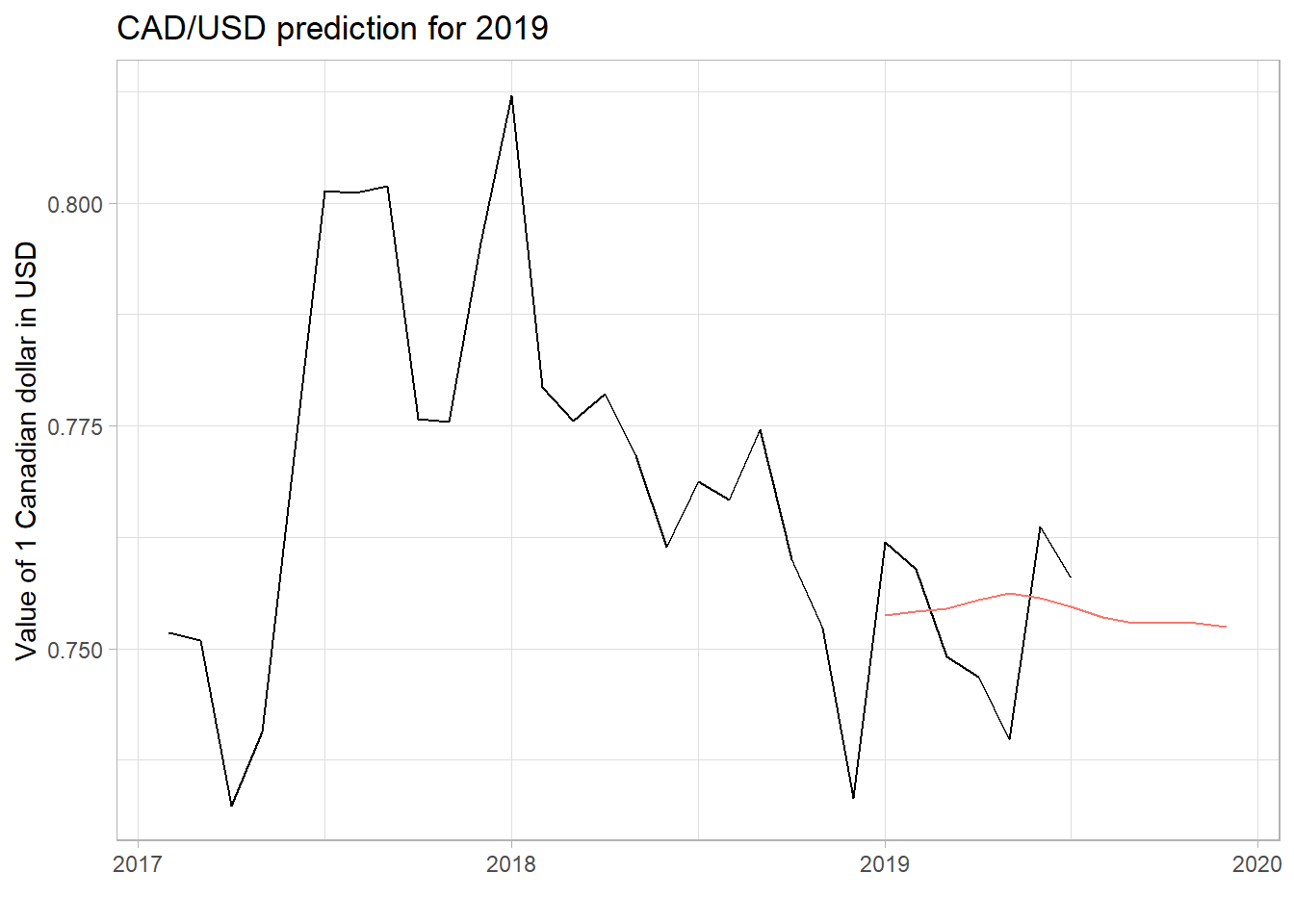
Figure 4: Oh well

Learning about the past and crunching numbers certainly does not give you the magical ability to see the future. However, I believe the value of technical analysis is in that it helps to understand finance from a concrete point of view, rather than from the abstract theories written more than half a century ago.

“To invest successfully, you need not understand beta, efficient markets, modern portfolio theory, option pricing or emerging markets. You may, in fact, be better off knowing nothing of these. That, of course, is not the prevailing view at most business schools, whose finance curriculum tends to be dominated by such subjects. In our view, though, investment students need only two well-taught courses - How to Value a Business, and How to Think About Market Prices.
- Warren Buffett”