
Predict Credit Default with Random Forest Model with Tuned Hyperparameters
I just want to focus on writing about implementing the workflow of this algorithm in R, so will keep the explanation very brief. However, these are some excellent articles that I referenced on hyperparameters, random forest and combining them.
Found this UCI Machine Learning Repo dataset containing Portuguese bank data from 2009. Its original focus was to determine how successful their marketing campaigns were (to get people to deposit money). But, it has a lot of variables that I wanted to use to tell another story with this dataset!
Background terminology
Random foreset
Random Forest is a classification/regression algorithm that makes use of many decision trees that act as a committee making decisions by majority vote. The most important detail is the uncorrelated-ness between trees. By creating many, many decision trees that don’t look like each other, the random forrest “hedges” risks of getting the wrong prediction. If one tree messes up, but many other trees with completely different features get it right, the initial tree is less guilty :) Much like a diversified investment portfolio. On top of this, to ensure even more randomness, decision crieria at each nodes of trees are decided by randomly chosen variables.
Tuning hyperparameters
Hyperparameters refer to the settings of a training process. These must be set by a human before training. In case of what we’re looking at today in a random forest,
- Number of trees
- Number of features allowed in nodes
- Minimum number of data points in a node that qualifies a split.
On the other hand, a parameter is something that a training process teaches itself, such as slope/intercept in linear models and coefficients in logistic models.
Grid search & cross validation
Kinda sounds very brute force-y, but tuning hyperparameters requires trying as many combinations possible and picking the best specs. To do this we’re going to use a technique called “Grid Search” to achieve this.
Finally, we’ll use resampling/subsampling methods like bootstrap or cross-validation to add randomness to the training dataset. I don’t quite fully understand the benefits/downsides of choosing one over the other, but I’m going to use cross-validation for this post.
Let’s build the model!
Quickly cleaned column names and gave row id’s.
library(tidyverse)
library(tidymodels)
theme_set(theme_light())

bank <- read_csv("bank_cleaned.csv") %>%
  janitor::clean_names() %>%
  rename(id = x1)

bank_rough <- bank %>%
  select(-response_binary) %>%
  mutate_if(is.character, factor)

bank_rough
## # A tibble: 40,841 x 17
## id age job marital education default balance housing loan day month
## <dbl> <dbl> <fct> <fct> <fct> <fct> <dbl> <fct> <fct> <dbl> <fct>
## 1 0 58 mana~ married tertiary no 2143 yes no 5 may
## 2 1 44 tech~ single secondary no 29 yes no 5 may
## 3 2 33 entr~ married secondary no 2 yes yes 5 may
## 4 5 35 mana~ married tertiary no 231 yes no 5 may
## 5 6 28 mana~ single tertiary no 447 yes yes 5 may
## 6 7 42 entr~ divorc~ tertiary yes 2 yes no 5 may
## 7 8 58 reti~ married primary no 121 yes no 5 may
## 8 9 43 tech~ single secondary no 593 yes no 5 may
## 9 10 41 admi~ divorc~ secondary no 270 yes no 5 may
## 10 11 29 admi~ single secondary no 390 yes no 5 may
## # ... with 40,831 more rows, and 6 more variables: duration <dbl>,
## # campaign <dbl>, pdays <dbl>, previous <dbl>, poutcome <fct>, response <fct>Quick EDA
This is something I like to do with numeric data. So I took all columns that are of class dbl, pivoted the dataframe, and then made a histogram for each variable.
bank_rough %>%
  select_if(is.double) %>%
  select(-id) %>%
  pivot_longer(age:previous) %>%
  ggplot(aes(value)) +
  geom_histogram() +
  facet_wrap(~name, scales = "free")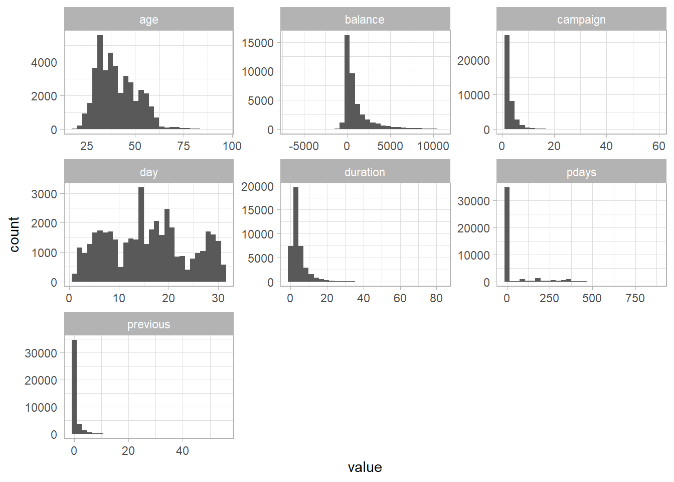
Interesting to see there’s negative balances, that’s probably gonna be a major predictor.
For the columns that weren’t selected, I’m going to do the exact same thing as above, but with column charts. This is a trick I learned recently. The powerful reorder_within & scale_y_reordered functions from the tidytext package makes it really easy to get a grasp our data.
library(tidytext)

bank_rough %>%
  select_if(is.factor) %>%
  mutate_all(as.character) %>%
  pivot_longer(job:response) %>%
  count(name, value) %>%
  mutate(value = reorder_within(value, n, name)) %>%
  ggplot(aes(n, value, fill = value)) +
  geom_col() +
  theme(legend.position = "none") +
  facet_wrap(~name, scales = "free") +
  scale_y_reordered()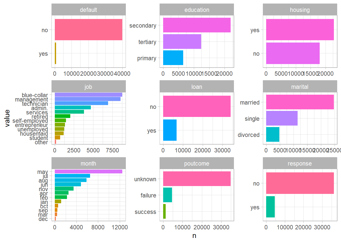
Now that we’ve seen all variables in this dataset, I’m going to take these variables that I think are important.
bank_proc <- bank_rough %>%
  select(id, education, default, housing, job, loan, marital, age, balance)
Model Building
Let’s set split our data into training/testing sets. “strata” argument just locks in the proportions of class, so that both training and testing sets have the same % mix of default and non-defaults.
library(tidymodels)
set.seed(123)

bank_split <- initial_split(bank_proc, strata = housing)
bank_train <- training(bank_split)
bank_test <- testing(bank_split)
I am going to tune our model twice. This tuning comes in after setting the recipe, algorithm specs, workflow, and then a cv-set. In the first tuning, I’m going to randomly select 20 combinations of hyperparameters (mtry and min_n), and then I’ll look at the result, and then narrow down the range of the combinations and tune once again. We’re going to do this the tidy way, with tidymodels. I’m excited to see what we can do with this!
1. Recipe
In tidymodels, a recipe works much like a cooking recipe. You first say what you’re going to cook (credit default explained by all variables from bank_train), and then add a bunch of “steps” you need to finish cooking. A recipe is not trained with any data yet, it’s just some specifications to the data before it’s fed into the model! Some steps we took are:
update_role: We just said theidcolumn is literally an id, so don’t use as a predictor.step_other: take a column, and an item within that column doesn’t come up frequently enough. I thought there were too many jobs, so we’ll lump the least frequent ones as “other”.step_dummy: turn every single item within each columns into a dummy variable.step_downsample: Make sure we have equal number of observations for credit defaults
bank_rec <- recipe(default ~ ., data = bank_train) %>%
  update_role(id, new_role = "id") %>%
  step_other(job, threshold = 0.03) %>%
  step_dummy(all_nominal(), -all_outcomes()) %>%
  step_downsample(default)
## Warning: `step_downsample()` was deprecated in recipes 0.1.13.
## Please use `themis::step_downsample()` instead.bank_prep <- prep(bank_rec)
juiced <- juice(bank_prep)This is what a recipe looks like. It’s just a preprocessing
bank_rec## Data Recipe
##
## Inputs:
##
## role #variables
## id 1
## outcome 1
## predictor 7
##
## Operations:
##
## Collapsing factor levels for job
## Dummy variables from all_nominal(), -all_outcomes()
## Down-sampling based on defaultA recipe needs to be prep’d, which gives us a summary
bank_prep## Data Recipe
##
## Inputs:
##
## role #variables
## id 1
## outcome 1
## predictor 7
##
## Training data contained 30631 data points and no missing data.
##
## Operations:
##
## Collapsing factor levels for job [trained]
## Dummy variables from education, housing, job, loan, marital [trained]
## Down-sampling based on default [trained]Then we can juice a recipe, which gives us the product of our instructions
juiced## # A tibble: 1,168 x 18
## id age balance default education_secon~ education_terti~ housing_yes
## <dbl> <dbl> <dbl> <fct> <dbl> <dbl> <dbl>
## 1 2023 31 606 no 0 1 1
## 2 42980 35 7050 no 0 1 0
## 3 28143 43 373 no 1 0 0
## 4 14981 37 764 no 1 0 1
## 5 21943 45 638 no 1 0 1
## 6 13692 42 199 no 0 1 1
## 7 10221 37 -119 no 0 1 1
## 8 441 34 242 no 0 1 1
## 9 2909 42 2535 no 1 0 1
## 10 8922 33 934 no 0 0 1
## # ... with 1,158 more rows, and 11 more variables: job_blue.collar <dbl>,
## # job_entrepreneur <dbl>, job_management <dbl>, job_retired <dbl>,
## # job_self.employed <dbl>, job_services <dbl>, job_technician <dbl>,
## # job_other <dbl>, loan_yes <dbl>, marital_married <dbl>,
## # marital_single <dbl>2. Algorithm Specs
Now we have to specify the settings of our random foreset. tune_spec is literally just a setting of a random forest we’re going to be applying. tune() means we’re going to tune this hyperparameter, so don’t specify just yet, like 100 for trees. (Would have done more than a 100, but it took forever so just doing 100) We’re tuning two hyperparams here:
- mtry: Number of features to be used to split a node
- min_n: Minimum number of items in a node that qualifies a split
And then, 2 final lines are saying we’re solving a classification problem with random forest, using a “ranger” package.
tune_spec <- rand_forest(
  mtry = tune(),
  trees = 100,
  min_n = tune()
) %>%
  set_mode("classification") %>%
  set_engine("ranger")
3. Workflow
Workflow puts everything together.
tune_wf <- workflow() %>%
  add_recipe(bank_rec) %>%
  add_model(tune_spec)

tune_wf
## == Workflow ====================================================================
## Preprocessor: Recipe
## Model: rand_forest()
##
## -- Preprocessor ----------------------------------------------------------------
## 3 Recipe Steps
##
## * step_other()
## * step_dummy()
## * step_downsample()
##
## -- Model -----------------------------------------------------------------------
## Random Forest Model Specification (classification)
##
## Main Arguments:
## mtry = tune()
## trees = 100
## min_n = tune()
##
## Computational engine: ranger4. Cross Validation and Grid Search Tuning
Now we make a 10-fold cross validation training sets
set.seed(234)
bank_folds <- vfold_cv(bank_train)

bank_folds
## # 10-fold cross-validation
## # A tibble: 10 x 2
## splits id
## <list> <chr>
## 1 <split [27.6K/3.1K]> Fold01
## 2 <split [27.6K/3.1K]> Fold02
## 3 <split [27.6K/3.1K]> Fold03
## 4 <split [27.6K/3.1K]> Fold04
## 5 <split [27.6K/3.1K]> Fold05
## 6 <split [27.6K/3.1K]> Fold06
## 7 <split [27.6K/3.1K]> Fold07
## 8 <split [27.6K/3.1K]> Fold08
## 9 <split [27.6K/3.1K]> Fold09
## 10 <split [27.6K/3.1K]> Fold10First Tuning
Now that we’ve established all the previous steps, let’s tune some hyperparameters
We turn on parallel processing to make it a bit faster, and use the tune_grid, which takes our workflow, cv set, and 20 random combinations of hyperparameters.
doParallel::registerDoParallel()

set.seed(345)
tune_res <- tune_grid(
  tune_wf,
  resamples = bank_folds,
  grid = 20
)
The result is a dataframe containing each data split we’re using to train, and the metrics.
tune_res## # Tuning results
## # 10-fold cross-validation
## # A tibble: 10 x 4
## splits id .metrics .notes
## <list> <chr> <list> <list>
## 1 <split [27.6K/3.1K]> Fold01 <tibble [40 x 6]> <tibble [0 x 1]>
## 2 <split [27.6K/3.1K]> Fold02 <tibble [40 x 6]> <tibble [0 x 1]>
## 3 <split [27.6K/3.1K]> Fold03 <tibble [40 x 6]> <tibble [0 x 1]>
## 4 <split [27.6K/3.1K]> Fold04 <tibble [40 x 6]> <tibble [0 x 1]>
## 5 <split [27.6K/3.1K]> Fold05 <tibble [40 x 6]> <tibble [0 x 1]>
## 6 <split [27.6K/3.1K]> Fold06 <tibble [40 x 6]> <tibble [0 x 1]>
## 7 <split [27.6K/3.1K]> Fold07 <tibble [40 x 6]> <tibble [0 x 1]>
## 8 <split [27.6K/3.1K]> Fold08 <tibble [40 x 6]> <tibble [0 x 1]>
## 9 <split [27.6K/3.1K]> Fold09 <tibble [40 x 6]> <tibble [0 x 1]>
## 10 <split [27.6K/3.1K]> Fold10 <tibble [40 x 6]> <tibble [0 x 1]>And we can pull the metrics like so:
tune_res %>%
  collect_metrics()
## # A tibble: 40 x 8
## mtry min_n .metric .estimator mean n std_err .config
## <int> <int> <chr> <chr> <dbl> <int> <dbl> <chr>
## 1 3 35 accuracy binary 0.758 10 0.00397 Preprocessor1_Model01
## 2 3 35 roc_auc binary 0.866 10 0.00696 Preprocessor1_Model01
## 3 12 19 accuracy binary 0.766 10 0.00526 Preprocessor1_Model02
## 4 12 19 roc_auc binary 0.869 10 0.00413 Preprocessor1_Model02
## 5 11 37 accuracy binary 0.765 10 0.00496 Preprocessor1_Model03
## 6 11 37 roc_auc binary 0.871 10 0.00514 Preprocessor1_Model03
## 7 13 20 accuracy binary 0.767 10 0.00466 Preprocessor1_Model04
## 8 13 20 roc_auc binary 0.869 10 0.00445 Preprocessor1_Model04
## 9 6 32 accuracy binary 0.763 10 0.00425 Preprocessor1_Model05
## 10 6 32 roc_auc binary 0.870 10 0.00582 Preprocessor1_Model05
## # ... with 30 more rowsLet’s pick the best hyperparameters according to roc_auc.
tune_res %>%
  collect_metrics() %>%
  filter(.metric == "roc_auc") %>%
  pivot_longer(mtry:min_n) %>%
  ggplot(aes(value, mean, color = name)) +
  geom_point() +
  geom_line() +
  facet_wrap(~name)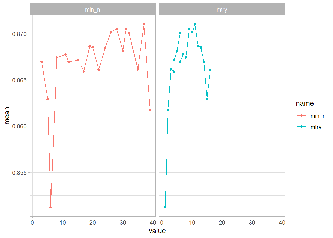
It seems like min_n is the most accurate around 5 & 10, while mtry was around 25, 35. Now that we know a little better, let’s try a bunch of combinations in those ranges to train our model!
Second Tuning
We need a new “grid”. We’re going to give it the ranges we want to test, and levels, which controls the number of possible combinations (trying too many would take too long!)
rf_grid <- grid_regular(
  mtry(range = c(5, 15)),
  min_n(range = c(25, 35)),
  levels = 10
)

rf_grid
## # A tibble: 100 x 2
## mtry min_n
## <int> <int>
## 1 5 25
## 2 6 25
## 3 7 25
## 4 8 25
## 5 9 25
## 6 10 25
## 7 11 25
## 8 12 25
## 9 13 25
## 10 15 25
## # ... with 90 more rowsSame exact tuning as the first one, but with a different grid.
set.seed(456)
regular_res <- tune_grid(
  tune_wf,
  resamples = bank_folds,
  grid = rf_grid
)

regular_res
## # Tuning results
## # 10-fold cross-validation
## # A tibble: 10 x 4
## splits id .metrics .notes
## <list> <chr> <list> <list>
## 1 <split [27.6K/3.1K]> Fold01 <tibble [200 x 6]> <tibble [0 x 1]>
## 2 <split [27.6K/3.1K]> Fold02 <tibble [200 x 6]> <tibble [0 x 1]>
## 3 <split [27.6K/3.1K]> Fold03 <tibble [200 x 6]> <tibble [0 x 1]>
## 4 <split [27.6K/3.1K]> Fold04 <tibble [200 x 6]> <tibble [0 x 1]>
## 5 <split [27.6K/3.1K]> Fold05 <tibble [200 x 6]> <tibble [0 x 1]>
## 6 <split [27.6K/3.1K]> Fold06 <tibble [200 x 6]> <tibble [0 x 1]>
## 7 <split [27.6K/3.1K]> Fold07 <tibble [200 x 6]> <tibble [0 x 1]>
## 8 <split [27.6K/3.1K]> Fold08 <tibble [200 x 6]> <tibble [0 x 1]>
## 9 <split [27.6K/3.1K]> Fold09 <tibble [200 x 6]> <tibble [0 x 1]>
## 10 <split [27.6K/3.1K]> Fold10 <tibble [200 x 6]> <tibble [0 x 1]>Let’s take a look at our results. This graph tells you the accuracy of models with specified hyperparameters where each line represents a min_n, and the x-axis represents mtry.
regular_res %>%
  collect_metrics() %>%
  filter(.metric == "roc_auc") %>%
  mutate(min_n = factor(min_n)) %>%
  select(mtry, min_n, mean) %>%
  ggplot(aes(mtry, mean, color = min_n)) +
  geom_point() +
  geom_line(alpha = 0.5, size = 1.5)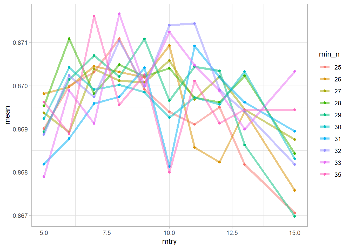
Seems like min_n of 35, at 8 mtry did the best. However, let’s not guess, there is a function for that!
best_auc <- select_best(regular_res, "roc_auc")

best_auc
## # A tibble: 1 x 3
## mtry min_n .config
## <int> <int> <chr>
## 1 8 33 Preprocessor1_Model0848 & 33 it is! Let’s finalize that.
final_rf <- finalize_model(
  tune_spec,
  best_auc
)

final_rf
## Random Forest Model Specification (classification)
##
## Main Arguments:
## mtry = 8
## trees = 100
## min_n = 33
##
## Computational engine: rangerTest model on test set
vip package lets us see how each variable affected the model. The way it does it is by looking at each decision nodes’ improvement compared to other nodes.
library(vip)##
## Attaching package: 'vip'## The following object is masked from 'package:utils':
##
## vifinal_rf %>%
set_engine("ranger", importance = "permutation") %>%
fit(default ~ .,
data = juice(bank_prep) %>% select(-id)
) %>%
vip(geom = "point")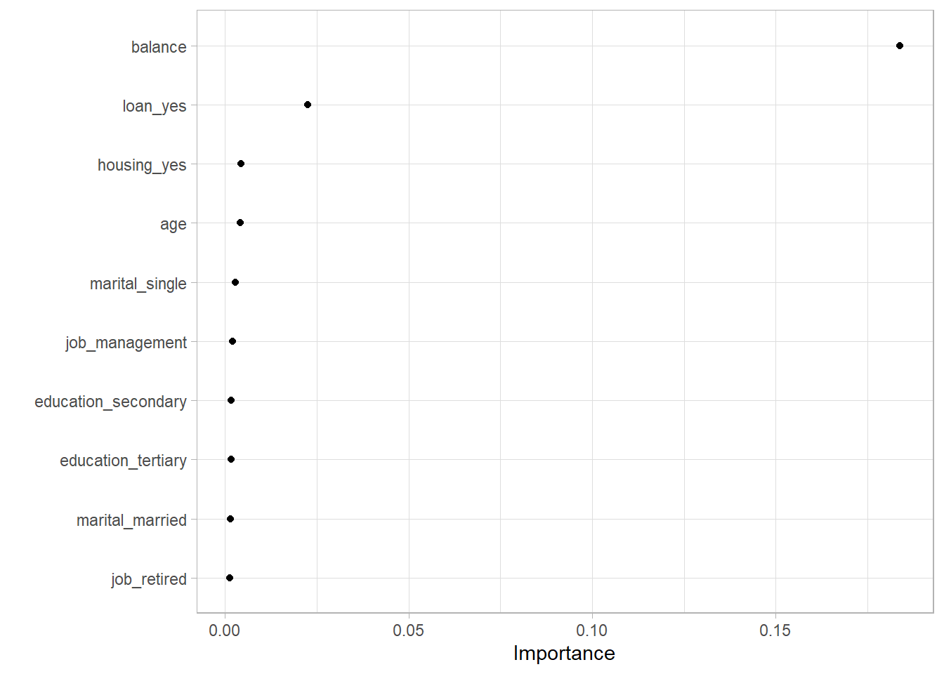
Obviously, your bank balance and whether you have loans or not will be a good predictor of credit default. All others seem meh though. That’s probably a problem. Maybe this model will be useless when an unseen relationship between bank balance and credit default shows up. But regardless, we’ll go forward.
We’re doing the exact same thing as above recipe, but with our final model.
final_wf <- workflow() %>%
  add_recipe(bank_rec) %>%
  add_model(final_rf)

final_res <- final_wf %>%
  last_fit(bank_split)

final_res
## # Resampling results
## # Manual resampling
## # A tibble: 1 x 6
## splits id .metrics .notes .predictions .workflow
## <list> <chr> <list> <list> <list> <list>
## 1 <split [30.6K~ train/test~ <tibble [2 ~ <tibble [0~ <tibble [10,210~ <workflo~76% accuracy. I think that’s pretty good.
final_res %>%
  collect_metrics()
## # A tibble: 2 x 4
## .metric .estimator .estimate .config
## <chr> <chr> <dbl> <chr>
## 1 accuracy binary 0.756 Preprocessor1_Model1
## 2 roc_auc binary 0.865 Preprocessor1_Model1One last thing to look at is the confusion matrix.
final_res %>%
  collect_predictions() %>%
  conf_mat(.pred_class, default)
## Truth
## Prediction no yes
## no 7568 2463
## yes 27 152Seems like it did a good job predicting when someone has not defaulted on their loan, but it also said a lot of no’s when in fact the person has defaulted on their loan. (lots of false positives)