
Cross-Checking Two Versions of Budget Files
Thanks Marc for reminding me to write!
Hey everyone, hope you’re all doing well! Lately, I’ve been spending most of my free time learning to make website designs with CSS. Some people rip of CSS for not being a real programming language, but it’s a tricky language to master! Unlike other languages like Python, with CSS, you really don’t know when something went wrong, unless you understand exactly what the impact of adding an extra line of code will do. This slows me down often, but oh well ¯\(ツ)/¯
Let’s get into it!
Today, I wanted to share a trick that really saved me a ton of time at work. Without going into too much detail, the task was to verify a file that contains a series of yearly budget numbers against another file that has similar information.
Seems pretty simple right? Sort the numbers by month, line them up next to each other, and do a “this cell equals that cell” formula, and drag it down?

While the first file was in a beautiful format, unfortunately the other one was just too messy for me to select all numbers at once.
Let me illustrate what I mean.
Data
Let’s say we’re looking at next year’s sales quota and forecast at different cities. I’ve set up 5 cities from 2 provinces, with some random data, so we have something to work with. This is my preferred format for pretty much anything. If all data was like this, I probably wouldn’t have a job lol
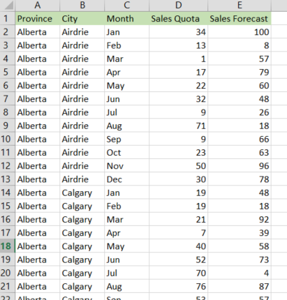
Figure 1: Beautifully formatted sheet
Now look at this sheet. This is what most pivot tables look like, with Province & City as rows, Month as columns, and Sales Quota & Sales Forecast as values. I’ve changed a couple numbers without thinking, so we got some work ahead of us, detecting where they are!
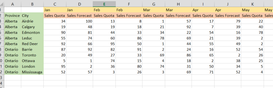
Figure 2: Wide-form sheet
The worksheet given to me was a tad messier than this, but you get the idea.
Processing
“wHy dON’t yOu jUsT uSe pIvOtTAblE?”
idk, I love using R to solve business problems.
Load data into R
I’m only gonna use 2 packages. openxlsx to open Excel, and tidyverse to wrangle.
library(openxlsx)
library(tidyverse)
Make sure you set the skipEmptyRows & skipEmptyCols to FALSE. Pretty dumb, but the default value is TRUE, so it really throws you off if you’re not aware.
I like using clean_names() so that all column names are just one word.
sheet1 <- read.xlsx("sheet1.xlsx", skipEmptyRows = FALSE, skipEmptyCols = FALSE) %>%
  janitor::clean_names()

sheet1 %>% head(10)
## province city month sales_quota sales_forecast
## 1 Alberta Airdrie Jan 34 100
## 2 Alberta Airdrie Feb 13 8
## 3 Alberta Airdrie Mar 1 57
## 4 Alberta Airdrie Apr 17 79
## 5 Alberta Airdrie May 22 60
## 6 Alberta Airdrie Jun 32 48
## 7 Alberta Airdrie Jul 9 26
## 8 Alberta Airdrie Aug 71 18
## 9 Alberta Airdrie Sep 9 66
## 10 Alberta Airdrie Oct 23 63I really wish there was something like head() for columns, but for now, I’ll just print the whole thing
sheet2 <- read.xlsx("sheet2.xlsx", skipEmptyRows = FALSE, skipEmptyCols = FALSE)

sheet2
## X1 X2 Jan Jan Feb Feb
## 1 Province City Sales Quota Sales Forecast Sales Quota Sales Forecast
## 2 Alberta Airdrie 34 100 13 8
## 3 Alberta Calgary 19 48 19 18
## 4 Alberta Edmonton 90 <NA> 44 33
## 5 Alberta Leduc 55 74 <NA> 86
## 6 Alberta Red Deer 92 66 95 50
## 7 Ontario Barrie 87 92 82 91
## 8 Ontario Toronto 52 57 52 26
## 9 Ontario Ottawa 95 40 36 80
## 10 Ontario London 20 49 26 33
## 11 Ontario Mississauga 5 71 74 151
## Mar Mar Apr Apr May
## 1 Sales Quota Sales Forecast Sales Quota Sales Forecast Sales Quota
## 2 1 57 17 79 22
## 3 21 92 7 39 40
## 4 <NA> 22 54 16 78
## 5 78 69 21 39 2
## 6 1 44 55 49 2
## 7 2 24 16 52 54
## 8 3 69 71 52 89
## 9 74 31 48 34 5
## 10 69 <NA> 65 76 26
## 11 14 18 <NA> 38 25
## May Jun Jun Jul Jul
## 1 Sales Forecast Sales Quota Sales Forecast Sales Quota Sales Forecast
## 2 60 32 48 9 26
## 3 58 52 73 70 4
## 4 <NA> 3 4 60 3
## 5 11 24 56 92 24
## 6 13 49 14 <NA> 56
## 7 63 42 67 42 91
## 8 19 31 15 55 40
## 9 2 <NA> 67 3 26
## 10 52 34 35 <NA> 56
## 11 33 27 8 64 38
## Aug Aug Sep Sep Oct
## 1 Sales Quota Sales Forecast Sales Quota Sales Forecast Sales Quota
## 2 71 18 9 66 23
## 3 76 87 53 57 61
## 4 64 43 31 2 12
## 5 58 30 44 35 39
## 6 56 19 98 50 35
## 7 97 30 20 18 76
## 8 19 28 49 22 <NA>
## 9 67 67 <NA> <NA> 81
## 10 1 61 44 30 67
## 11 6 15 29 9 <NA>
## Oct Nov Nov Dec Dec
## 1 Sales Forecast Sales Quota Sales Forecast Sales Quota Sales Forecast
## 2 63 50 96 30 78
## 3 43 <NA> 84 57 72
## 4 1 40 2 50 94
## 5 <NA> 30 1 30 78
## 6 52 58 <NA> 2 64
## 7 78 24 32 90 85
## 8 46 30 40 17 3
## 9 49 40 29 54 <NA>
## 10 36 4 40 <NA> 1
## 11 2 99 54 92 24Sheet1 Clean
Not much to clean here, but I’ll turn all my numbers (quota & forecast) into a key-value format. This will be useful when we make charts later!
sheet1 <- sheet1 %>%
  gather(type, value, -c(province, city, month))

sheet1 %>% head(10)
## province city month type value
## 1 Alberta Airdrie Jan sales_quota 34
## 2 Alberta Airdrie Feb sales_quota 13
## 3 Alberta Airdrie Mar sales_quota 1
## 4 Alberta Airdrie Apr sales_quota 17
## 5 Alberta Airdrie May sales_quota 22
## 6 Alberta Airdrie Jun sales_quota 32
## 7 Alberta Airdrie Jul sales_quota 9
## 8 Alberta Airdrie Aug sales_quota 71
## 9 Alberta Airdrie Sep sales_quota 9
## 10 Alberta Airdrie Oct sales_quota 23You kinda see what’s going on here, the column names are in the “type” column, and the corresponding value is in the “value” column. If I printed the end of this, it’ll show sales_forecast too. Like so:
sheet1 %>% tail(10)## province city month type value
## 231 Ontario Mississauga Mar sales_forecast 18
## 232 Ontario Mississauga Apr sales_forecast 38
## 233 Ontario Mississauga May sales_forecast 33
## 234 Ontario Mississauga Jun sales_forecast 8
## 235 Ontario Mississauga Jul sales_forecast 38
## 236 Ontario Mississauga Aug sales_forecast 15
## 237 Ontario Mississauga Sep sales_forecast 9
## 238 Ontario Mississauga Oct sales_forecast 5
## 239 Ontario Mississauga Nov sales_forecast 54
## 240 Ontario Mississauga Dec sales_forecast 88This is all I’m going to do! Let’s turn sheet2 like this
Sheet2 Clean
Remember how sheet2 looked like up top? I’ll print the first few columns, now that you know what it looks like, no point wasting space. When you see the below code popping up again, I’m just printing the first 6 columns.
sheet2[, 1:6]## X1 X2 Jan Jan.1 Feb Feb.1
## 1 Province City Sales Quota Sales Forecast Sales Quota Sales Forecast
## 2 Alberta Airdrie 34 100 13 8
## 3 Alberta Calgary 19 48 19 18
## 4 Alberta Edmonton 90 <NA> 44 33
## 5 Alberta Leduc 55 74 <NA> 86
## 6 Alberta Red Deer 92 66 95 50
## 7 Ontario Barrie 87 92 82 91
## 8 Ontario Toronto 52 57 52 26
## 9 Ontario Ottawa 95 40 36 80
## 10 Ontario London 20 49 26 33
## 11 Ontario Mississauga 5 71 74 151Column Names
I really don’t like how the first two column names are useless (X1, X2). These are just random names that R assigns when there is no column name explicitly specified.
Let’s get rid of them. The idea is to combine the column names and the first row together, set that as the column name, and get rid of the first row.
new_col_names <- paste(sheet2[1,], names(sheet2), sep = "-")

new_col_names
## [1] "Province-X1" "City-X2" "Sales Quota-Jan"
## [4] "Sales Forecast-Jan" "Sales Quota-Feb" "Sales Forecast-Feb"
## [7] "Sales Quota-Mar" "Sales Forecast-Mar" "Sales Quota-Apr"
## [10] "Sales Forecast-Apr" "Sales Quota-May" "Sales Forecast-May"
## [13] "Sales Quota-Jun" "Sales Forecast-Jun" "Sales Quota-Jul"
## [16] "Sales Forecast-Jul" "Sales Quota-Aug" "Sales Forecast-Aug"
## [19] "Sales Quota-Sep" "Sales Forecast-Sep" "Sales Quota-Oct"
## [22] "Sales Forecast-Oct" "Sales Quota-Nov" "Sales Forecast-Nov"
## [25] "Sales Quota-Dec" "Sales Forecast-Dec"Now that we have the new column names, let’s set this list as the column names, and get rid of the first row. (Second row to last row)
names(sheet2) <- new_col_names

sheet2 <- sheet2[2:nrow(sheet2),]

sheet2[, 1:6]
## Province-X1 City-X2 Sales Quota-Jan Sales Forecast-Jan Sales Quota-Feb
## 2 Alberta Airdrie 34 100 13
## 3 Alberta Calgary 19 48 19
## 4 Alberta Edmonton 90 <NA> 44
## 5 Alberta Leduc 55 74 <NA>
## 6 Alberta Red Deer 92 66 95
## 7 Ontario Barrie 87 92 82
## 8 Ontario Toronto 52 57 52
## 9 Ontario Ottawa 95 40 36
## 10 Ontario London 20 49 26
## 11 Ontario Mississauga 5 71 74
## Sales Forecast-Feb
## 2 8
## 3 18
## 4 33
## 5 86
## 6 50
## 7 91
## 8 26
## 9 80
## 10 33
## 11 151I’m going to manipulate the column names later on except the first two, so might as well clean the good ones now.
names(sheet2)[1:2] <- c("province", "city")

sheet2[, 1:6]
## province city Sales Quota-Jan Sales Forecast-Jan Sales Quota-Feb
## 2 Alberta Airdrie 34 100 13
## 3 Alberta Calgary 19 48 19
## 4 Alberta Edmonton 90 <NA> 44
## 5 Alberta Leduc 55 74 <NA>
## 6 Alberta Red Deer 92 66 95
## 7 Ontario Barrie 87 92 82
## 8 Ontario Toronto 52 57 52
## 9 Ontario Ottawa 95 40 36
## 10 Ontario London 20 49 26
## 11 Ontario Mississauga 5 71 74
## Sales Forecast-Feb
## 2 8
## 3 18
## 4 33
## 5 86
## 6 50
## 7 91
## 8 26
## 9 80
## 10 33
## 11 151Extract and Transform (The dreaded buzzword “ETL” haha!)
We still haven’t created “month”, “type” columns like sheet1 😢 Or, if you’re a cup-is-half-full type person, at least we’ve got “province” & “city” columns! 😄
This is exactly what leads into the next step. Let’s turn everything else that is not “province”, or “city”, into a key-value format. Here are the first 25 rows.
sheet2 <- sheet2 %>%
  gather(key, value, -c(province, city))

sheet2 %>% head(25)
## province city key value
## 1 Alberta Airdrie Sales Quota-Jan 34
## 2 Alberta Calgary Sales Quota-Jan 19
## 3 Alberta Edmonton Sales Quota-Jan 90
## 4 Alberta Leduc Sales Quota-Jan 55
## 5 Alberta Red Deer Sales Quota-Jan 92
## 6 Ontario Barrie Sales Quota-Jan 87
## 7 Ontario Toronto Sales Quota-Jan 52
## 8 Ontario Ottawa Sales Quota-Jan 95
## 9 Ontario London Sales Quota-Jan 20
## 10 Ontario Mississauga Sales Quota-Jan 5
## 11 Alberta Airdrie Sales Forecast-Jan 100
## 12 Alberta Calgary Sales Forecast-Jan 48
## 13 Alberta Edmonton Sales Forecast-Jan <NA>
## 14 Alberta Leduc Sales Forecast-Jan 74
## 15 Alberta Red Deer Sales Forecast-Jan 66
## 16 Ontario Barrie Sales Forecast-Jan 92
## 17 Ontario Toronto Sales Forecast-Jan 57
## 18 Ontario Ottawa Sales Forecast-Jan 40
## 19 Ontario London Sales Forecast-Jan 49
## 20 Ontario Mississauga Sales Forecast-Jan 71
## 21 Alberta Airdrie Sales Quota-Feb 13
## 22 Alberta Calgary Sales Quota-Feb 19
## 23 Alberta Edmonton Sales Quota-Feb 44
## 24 Alberta Leduc Sales Quota-Feb <NA>
## 25 Alberta Red Deer Sales Quota-Feb 95Here’s the beauty of processing.
We separate the key column into two new columns, by splitting the -
sheet2 <- sheet2 %>%
  separate(key, into = c("type", "month"), sep = "\\-")

sheet2 %>% head(10)
## province city type month value
## 1 Alberta Airdrie Sales Quota Jan 34
## 2 Alberta Calgary Sales Quota Jan 19
## 3 Alberta Edmonton Sales Quota Jan 90
## 4 Alberta Leduc Sales Quota Jan 55
## 5 Alberta Red Deer Sales Quota Jan 92
## 6 Ontario Barrie Sales Quota Jan 87
## 7 Ontario Toronto Sales Quota Jan 52
## 8 Ontario Ottawa Sales Quota Jan 95
## 9 Ontario London Sales Quota Jan 20
## 10 Ontario Mississauga Sales Quota Jan 5OK! It looks really similar to sheet1 now.
Final touches
Just a couple more steps left in processing. Let’s remind ourselves what sheet1 looks like
sheet1 %>% head(10)## province city month type value
## 1 Alberta Airdrie Jan sales_quota 34
## 2 Alberta Airdrie Feb sales_quota 13
## 3 Alberta Airdrie Mar sales_quota 1
## 4 Alberta Airdrie Apr sales_quota 17
## 5 Alberta Airdrie May sales_quota 22
## 6 Alberta Airdrie Jun sales_quota 32
## 7 Alberta Airdrie Jul sales_quota 9
## 8 Alberta Airdrie Aug sales_quota 71
## 9 Alberta Airdrie Sep sales_quota 9
## 10 Alberta Airdrie Oct sales_quota 23We need to clean the word “Sales Quota”, and “Sales Forecast” into lowercase
sheet2 <- sheet2 %>%
  mutate(type = str_replace(tolower(type), "\\s", "\\_"))

sheet2 %>% head(10)
## province city type month value
## 1 Alberta Airdrie sales_quota Jan 34
## 2 Alberta Calgary sales_quota Jan 19
## 3 Alberta Edmonton sales_quota Jan 90
## 4 Alberta Leduc sales_quota Jan 55
## 5 Alberta Red Deer sales_quota Jan 92
## 6 Ontario Barrie sales_quota Jan 87
## 7 Ontario Toronto sales_quota Jan 52
## 8 Ontario Ottawa sales_quota Jan 95
## 9 Ontario London sales_quota Jan 20
## 10 Ontario Mississauga sales_quota Jan 5Also, I’m going to change the name of the column “value” into something that is not “value”, because that name already exists in sheet1, so it collides when they join, as you’ll see.
sheet2 <- sheet2 %>%
  rename(sheet2_value = value)

sheet2 %>% head(10)
## province city type month sheet2_value
## 1 Alberta Airdrie sales_quota Jan 34
## 2 Alberta Calgary sales_quota Jan 19
## 3 Alberta Edmonton sales_quota Jan 90
## 4 Alberta Leduc sales_quota Jan 55
## 5 Alberta Red Deer sales_quota Jan 92
## 6 Ontario Barrie sales_quota Jan 87
## 7 Ontario Toronto sales_quota Jan 52
## 8 Ontario Ottawa sales_quota Jan 95
## 9 Ontario London sales_quota Jan 20
## 10 Ontario Mississauga sales_quota Jan 5That’s it for processing raw inputs. Checking their dimensions give us the mental check.
dim(sheet1)## [1] 240 5dim(sheet2)## [1] 240 5Join Two Tables
I recommend left-joining the bigger set with the smaller set. In this scenario, there’s no discrepancy btw tow tables. So I can use inner-join, but I’m still gonna use left-join.
joined <- sheet1 %>%
  left_join(sheet2, by = c("province", "city", "type", "month"))

joined %>% head(10)
## province city month type value sheet2_value
## 1 Alberta Airdrie Jan sales_quota 34 34
## 2 Alberta Airdrie Feb sales_quota 13 13
## 3 Alberta Airdrie Mar sales_quota 1 1
## 4 Alberta Airdrie Apr sales_quota 17 17
## 5 Alberta Airdrie May sales_quota 22 22
## 6 Alberta Airdrie Jun sales_quota 32 32
## 7 Alberta Airdrie Jul sales_quota 9 9
## 8 Alberta Airdrie Aug sales_quota 71 71
## 9 Alberta Airdrie Sep sales_quota 9 9
## 10 Alberta Airdrie Oct sales_quota 23 23And Voila, we have a dataframe that has sheet1 value in one column, and sheet 2 value in the other column!
Now, if we make a column that checks if two values are equal to each other, we can count it, and do other stuff with it.
Also, let’s put in an iferror.
joined <- joined %>%
  mutate(is_match = value == sheet2_value,
         is_match = replace_na(is_match, FALSE))


joined %>% head(10)
## province city month type value sheet2_value is_match
## 1 Alberta Airdrie Jan sales_quota 34 34 TRUE
## 2 Alberta Airdrie Feb sales_quota 13 13 TRUE
## 3 Alberta Airdrie Mar sales_quota 1 1 TRUE
## 4 Alberta Airdrie Apr sales_quota 17 17 TRUE
## 5 Alberta Airdrie May sales_quota 22 22 TRUE
## 6 Alberta Airdrie Jun sales_quota 32 32 TRUE
## 7 Alberta Airdrie Jul sales_quota 9 9 TRUE
## 8 Alberta Airdrie Aug sales_quota 71 71 TRUE
## 9 Alberta Airdrie Sep sales_quota 9 9 TRUE
## 10 Alberta Airdrie Oct sales_quota 23 23 TRUENow we’re ready to make some analysis & viz!
Analysis and Visualization
First of all, how many are incorrect?
joined %>% summarize(mean(is_match == FALSE))## mean(is_match == FALSE)
## 1 0.220833322%! I must have changed a lot!
I might have talked about this already, but summarize -> mean -> boolean is a neat trick to count the percentage of rows that meet the boolean.
While we’re at is, let’s see wow many wrong’s were caused by missing values in the second sheet?
joined %>%
  filter(is_match == FALSE) %>%
  summarize(mean(is.na(sheet2_value)))
## mean(is.na(sheet2_value))
## 1 0.3396226This is super valuable info. It tells me “of the 22% discrepancies btw the two files, 34% come from missing data in the second file.”
Anyways, I like using count() to quickly cycle between visualizations. Some questions I might be asking myself are:
Q1: Where were the wrong’s?
A1: London and Edmonton.
theme_set(theme_light())

joined %>%
  filter(is_match == FALSE) %>%
  count(province, city) %>%
  mutate(city = fct_reorder(city, n)) %>%
  ggplot(aes(city, n, fill = province)) +
  geom_col() +
  coord_flip() +
  labs(title = "Inconsistency between two files",
       x = "City",
       y = "# Mismatches")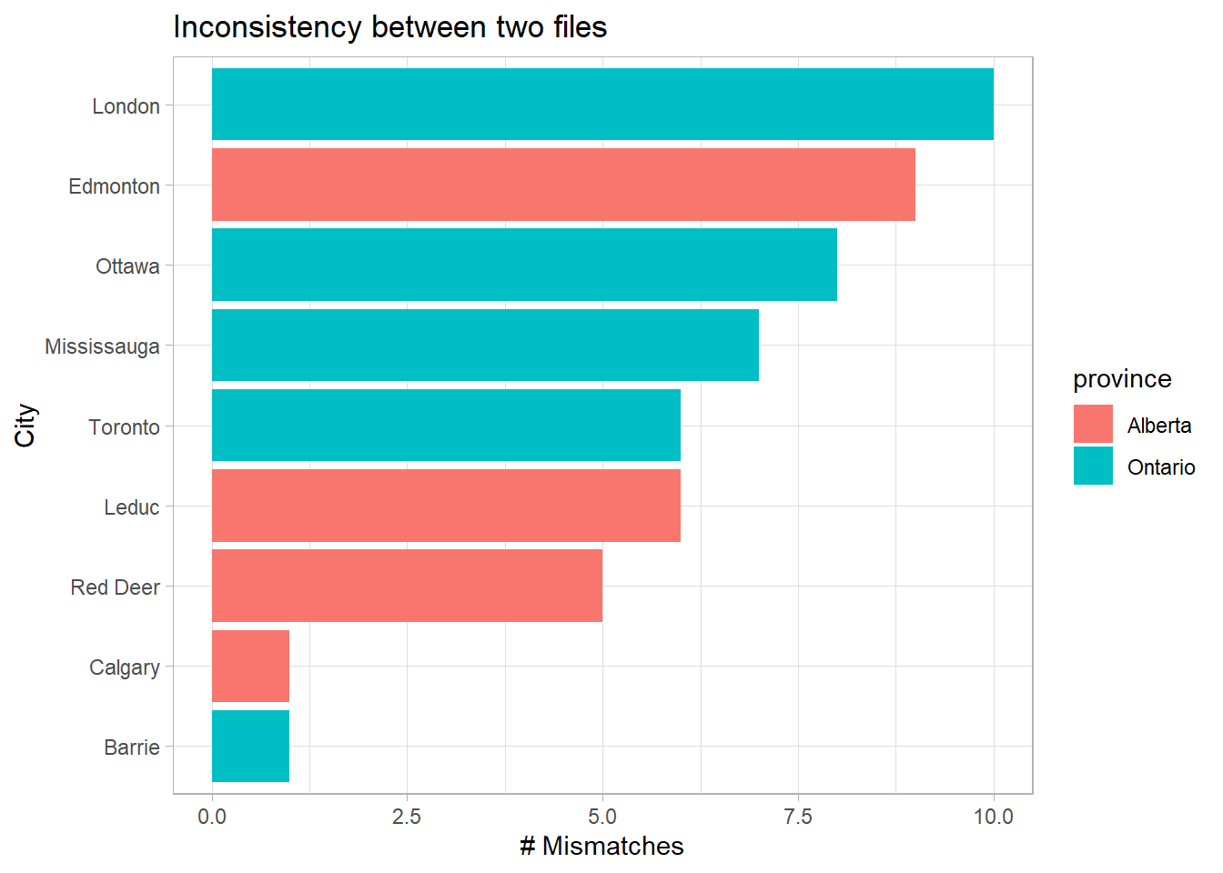
Q2: Was there a certain month that was forecast or budget wereparticularly wrong?
A2: Fourth quarter was brutal.
theme_set(theme_light())

joined %>%
  filter(is_match == FALSE) %>%
  count(month) %>%
  mutate(month = fct_reorder(month, n)) %>%
  ggplot(aes(month, n)) +
  geom_col() +
  coord_flip() +
  labs(title = "Inconsistency between two files",
       x = "Months",
       y = "# Mismatches")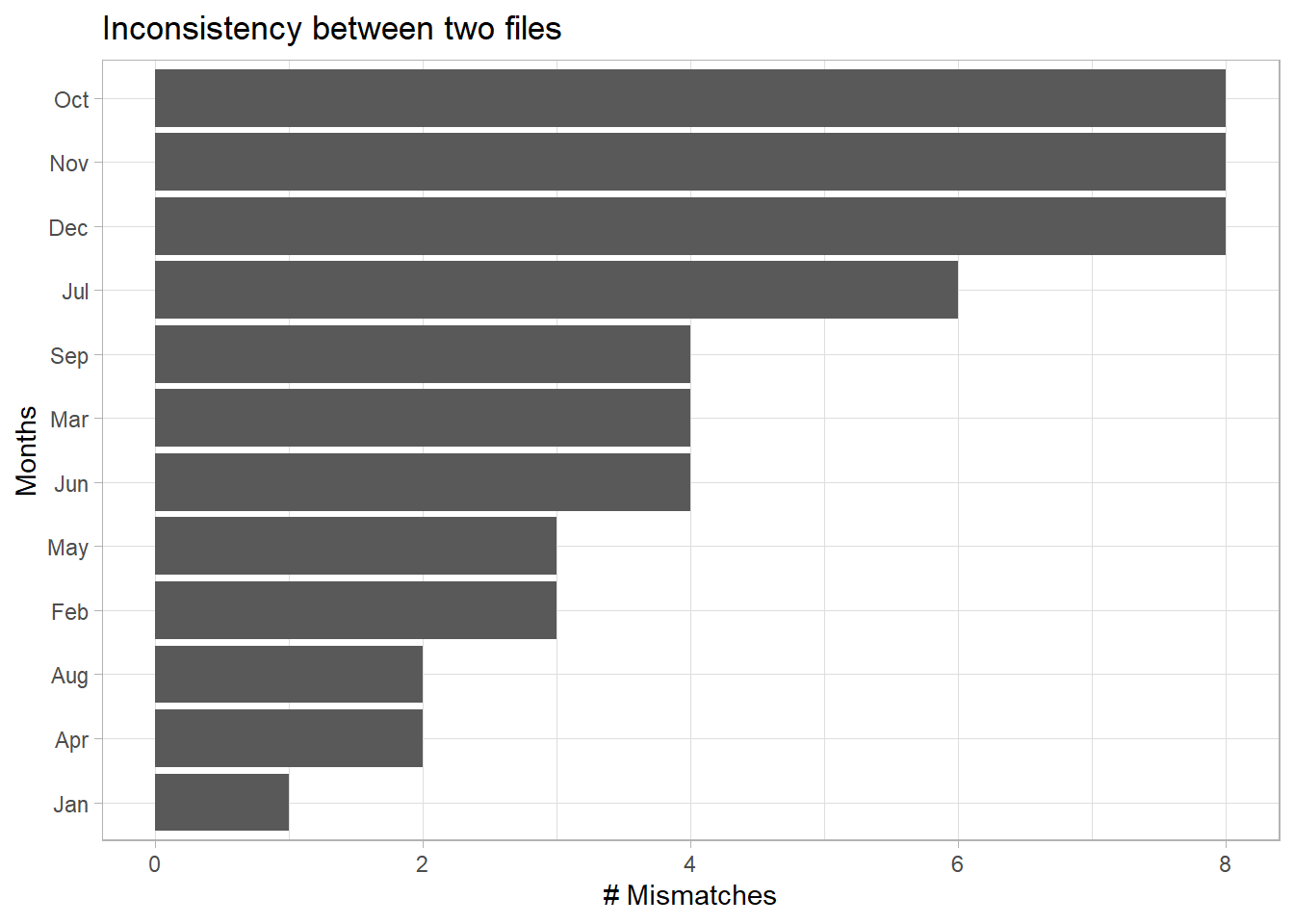
Conclusion
So yea, here’s how I would tackle these types of problems. A SQL-ly solution, that makes use of some of the beautiful functions in tidyverse!
I like this solution because once you set this up, and as long as the data format doesn’t change in either files, you can test a bunch of different files. Maybe you went back and filled in the missing values. Then, your accuracy goes up, and maybe then, you can focus on one city at a time.
Thanks for sticking around, I had a ton of fun doing this!