
Comparing Linear Regressions with Tidymodels
Hello! Today, we’re going to predict the costs of various transit projects around the world, by building 3 linear regression models. (simple linear regression, penalized regression, and partial least squares regression) Since we’re working with more than 1 model, we can actually compare the accuracies between different models, and see which might be the most suitable in this particular scenario!
The inspiration behind this post comes from the book “Applied Predictive Modeling” by RStudio’s Max Kuhn. He wrote this book a long time ago to demonstrate predictive modeling with the caret package, a meta machine learning library in R before the tidymodels family. (which he also is a major contributor in) Instead of following the old instructions, I thought it’d be fun to code the same statistical concepts with the great tidymodels package.
Data Reading & tldr;
This dataset was put together on January 5th TidyTuesday by the Transit Cost Project, and here’s their abstract behind the dataset:
Why do transit-infrastructure projects in New York cost 20 times more on a per kilometer basis than in Seoul? We investigate this question across hundreds of transit projects from around the world. We have created a database that spans more than 50 countries and totals more than 11,000 km of urban rail built since the late 1990s.
After reading the csv from github, I found the following variables interesting/informative and decided to use them to predict the real cost of transit line projects in millions of USD:
- Start Year
- End Year (therefore, also the duration of the project)
- Country
- Length of the transit line
- Tunnel length, if any
- Number of stations
library(tidyverse)

transit_cost <- readr::read_csv('https://raw.githubusercontent.com/rfordatascience/tidytuesday/master/data/2021/2021-01-05/transit_cost.csv') %>%
  filter(!start_year %in% c("4 years", "5 years", "not start") & !is.na(start_year)) %>%
  filter(!end_year %in% c("4 years", "5 years", "not start", "X") & !is.na(end_year)) %>%
  mutate(across(c(start_year, end_year, real_cost), ~as.numeric(.))) %>%
  select(id = e, start_year, end_year, country, length, tunnel, stations, real_cost) %>%
  mutate(duration = end_year - start_year) %>%
  mutate(across(c(tunnel, stations), ~ifelse(is.na(.), 0, .)))

transit_cost
## # A tibble: 462 x 9
## id start_year end_year country length tunnel stations real_cost duration
## <dbl> <dbl> <dbl> <chr> <dbl> <dbl> <dbl> <dbl> <dbl>
## 1 7136 2020 2025 CA 5.7 5 6 2377. 5
## 2 7137 2009 2017 CA 8.6 8.6 6 2592 8
## 3 7138 2020 2030 CA 7.8 7.8 3 4620 10
## 4 7139 2020 2030 CA 15.5 8.8 15 7201. 10
## 5 7144 2020 2030 CA 7.4 7.4 6 4704 10
## 6 7145 2003 2018 NL 9.7 7.1 8 4030 15
## 7 7146 2020 2026 CA 5.8 5.8 5 3780 6
## 8 7147 2009 2016 US 5.1 5.1 2 1756 7
## 9 7152 2020 2027 US 4.2 4.2 2 3600 7
## 10 7153 2018 2026 US 4.2 4.2 2 2400 8
## # ... with 452 more rowsI’m going to skip the EDA, for the sake of keeping the post length reasonable. Here’s the tldr of this post:
Model building
Let’s build some models! As usual, we’re going to split the data into training/testing sets, as well as bootstrap resampling to tune some hyperparameters later.
library(tidymodels)

set.seed(1234)
transit_initial_split <- initial_split(transit_cost)
transit_training <- training(transit_initial_split)
transit_testing <- testing(transit_initial_split)

set.seed(2345)
transit_boot <- bootstraps(transit_training)
Simple Linear Regression
Nothing too out of the usual in the recipe. We make the id column an id, so we don’t use it to train the model, normalize all the numeric predictors, step_other the countries, so we only take the countries with the most projects, and classify all as “others”. In our case, I went to the extreme, and selected 1 top country, China, and grouped all else as “others”, and then dummied it.
I recently learned by trial and error, that any pre-processing steps that involve the response variable, (real_cost) have a good chance of throwing off the testing set. This means I have to explicitly leave out the response, when using calls like all_numeric().
transit_rec <- recipe(real_cost ~ ., data = transit_training) %>%
  update_role(id, new_role = "id") %>%
  step_normalize(all_numeric(), -c(id, real_cost)) %>%
  step_other(country, threshold = 0.5) %>%
  step_dummy(country)
This pre-processing recipe will remain the same for all three models, that way we can see the differences in predictions due to model specs.
Next, we define the simple linear regression model specs, which doesn’t have any hyperparameters, so no arguments will be given to the linear_reg call. This will be a little different when we define the penalized model!
slr_spec <- linear_reg() %>%
  set_mode("regression") %>%
  set_engine("lm")
Now that we have the pre-processing recipe and a spec, we can train the model, and predict on the testing set! I really like carrying the two around in a workflow, because it’s easy to visualize the process from start to finish.
transit_wf <- workflow() %>%
  add_recipe(transit_rec) %>%
  add_model(slr_spec)

transit_wf
## == Workflow ====================================================================
## Preprocessor: Recipe
## Model: linear_reg()
##
## -- Preprocessor ----------------------------------------------------------------
## 3 Recipe Steps
##
## * step_normalize()
## * step_other()
## * step_dummy()
##
## -- Model -----------------------------------------------------------------------
## Linear Regression Model Specification (regression)
##
## Computational engine: lmThen, the training data is fit to the workflow, meaning it goes through the pre-processing recipe, and the modeling spec. With the trained workflow, we give it the new (testing) data, and predict the outcome, which is saved as slr_pred. Finally, we place the outcomes right next to its original data.
slr_pred <- transit_wf %>%
  fit(transit_training) %>%
  predict(transit_testing)

slr_pred %>%
  cbind(transit_testing) %>%
  head()
## .pred id start_year end_year country length tunnel stations real_cost
## 1 5084.2688 7139 2020 2030 CA 15.5 8.8 15 7201.32
## 2 2891.5977 7153 2018 2026 US 4.2 4.2 2 2400.00
## 3 507.9284 7168 2009 2012 BG 5.1 3.1 4 687.83
## 4 3890.9995 7170 2008 2012 BG 17.0 15.3 11 3160.64
## 5 1483.4923 7178 2010 2015 PL 6.5 6.5 7 3286.30
## 6 1602.6044 7209 2012 2021 IT 1.9 1.9 2 251.55
## duration
## 1 10
## 2 8
## 3 3
## 4 4
## 5 5
## 6 9Just for simplicity’s sake, we’re going to use R-squared to measure the robustness of the models.
slr_rsq <- slr_pred %>%
  cbind(transit_testing) %>%
  rsq(truth = real_cost, estimate = .pred) %>%
  select(.estimate) %>%
  mutate(model = "SLR")

slr_rsq
## # A tibble: 1 x 2
## .estimate model
## <dbl> <chr>
## 1 0.702 SLROK, one down!
Partial Lease Squares (PLS)
Much like PCA (principal component analysis), PLS seeks to reduce the dataset’s dimension by replacing numerous predictors with linear combinations of the predictors that explain the most variance in the predictors. The difference is that in PLS, it simultaneously searches the linear combinations of predictors that also minimizes the outcome.
While we don’t have a ton of predictors to begin with, this model offers something different from your everyday linear regression models. Since we’re not going to change the recipe, we simply need to define another model spec, and update the workflow. Notice the change in the model. It has one hyper parameter, num_comp, which I’ve arbitrarily set to 3. I could have tuned it to find the optimal number, but wanted to save the hyperparameter tuning until the next section!
library(plsmod)
pls_spec <- pls(num_comp = 3) %>%
  set_mode("regression") %>%
  set_engine("mixOmics")

transit_wf <- transit_wf %>% update_model(pls_spec)

transit_wf
## == Workflow ====================================================================
## Preprocessor: Recipe
## Model: pls()
##
## -- Preprocessor ----------------------------------------------------------------
## 3 Recipe Steps
##
## * step_normalize()
## * step_other()
## * step_dummy()
##
## -- Model -----------------------------------------------------------------------
## PLS Model Specification (regression)
##
## Main Arguments:
## num_comp = 3
##
## Computational engine: mixOmicsAnd then, we’re just repeating the steps above, of fitting the training set, predicting the testing set, and calculating the R-squared.
pls_pred <- transit_wf %>%
  fit(transit_training) %>%
  predict(transit_testing)

pls_rsq <- pls_pred %>%
  cbind(transit_testing) %>%
  rsq(truth = real_cost, estimate = .pred) %>%
  select(.estimate) %>%
  mutate(model = "PLS")

pls_rsq
## # A tibble: 1 x 2
## .estimate model
## <dbl> <chr>
## 1 0.668 PLSThat’s it for PLS, pretty short huh? I can’t stress enough how easy it is to swap out different aspects of model building with tidymodels!!!!! Many thanks to all brilliant minds at the tidymodels team :)
If I really wanted to, I can write a custom function that does the fit, predict, cbind, and rsq all in one. (Or maybe there’s already something out there, I know there’s workflowsets package that I haven’t tried yet)
Penalized Model
The post is getting a little long, but if you’re still reading, you’re probably with me until the end, so buckle in! :)
I like the penalized regression model because it discourages a simple linear regression from overfitting the training dataset, by introducing artificial penalties. There are two ways of applying the penalties, ridge, and lasso. Evidently, the amount of penalty, as well as the mixture of ridge/lasso are the two “hyperparameters” of the penalized model that you can set to achieve different results. (mixture ranges from 0 to 1, with 1 being lasso, 0 being ridge, and anything inbetween is a combination of the two) Here’s a good YouTube video.
We’re going to tune these hyperparameters to optimize the model performance.
The initial setup is the same.
penalized_spec <- linear_reg(mixture = tune(), penalty = tune()) %>%
  set_mode("regression") %>%
  set_engine("glmnet")

transit_wf <- transit_wf %>% update_model(penalized_spec)

transit_wf
## == Workflow ====================================================================
## Preprocessor: Recipe
## Model: linear_reg()
##
## -- Preprocessor ----------------------------------------------------------------
## 3 Recipe Steps
##
## * step_normalize()
## * step_other()
## * step_dummy()
##
## -- Model -----------------------------------------------------------------------
## Linear Regression Model Specification (regression)
##
## Main Arguments:
## penalty = tune()
## mixture = tune()
##
## Computational engine: glmnetpenalized_search is just a combination of the two parameters that we can use to train the model. In our case, we have 25 combinations.
penalized_search <- grid_regular(parameters(mixture(), penalty()), levels = 5)

penalized_search
## # A tibble: 25 x 2
## mixture penalty
## <dbl> <dbl>
## 1 0 0.0000000001
## 2 0.25 0.0000000001
## 3 0.5 0.0000000001
## 4 0.75 0.0000000001
## 5 1 0.0000000001
## 6 0 0.0000000316
## 7 0.25 0.0000000316
## 8 0.5 0.0000000316
## 9 0.75 0.0000000316
## 10 1 0.0000000316
## # ... with 15 more rowsTurn on parallel processing to speed up the training, and we use the bootstrap resamples to validate the accuracy. I write about the bootstrap resampling method in this post.
The tuned results come in a 25-row dataframe, for 25 combinations of hyperparameters, and each has its own train/test split, as well as various metrics for accuracies.
doParallel::registerDoParallel()
penalized_tune <- tune_grid(
  transit_wf,
  resamples = transit_boot,
  grid = penalized_search
)

penalized_tune
## # Tuning results
## # Bootstrap sampling
## # A tibble: 25 x 4
## splits id .metrics .notes
## <list> <chr> <list> <list>
## 1 <split [347/129]> Bootstrap01 <tibble [50 x 6]> <tibble [0 x 1]>
## 2 <split [347/137]> Bootstrap02 <tibble [50 x 6]> <tibble [0 x 1]>
## 3 <split [347/129]> Bootstrap03 <tibble [50 x 6]> <tibble [0 x 1]>
## 4 <split [347/121]> Bootstrap04 <tibble [50 x 6]> <tibble [0 x 1]>
## 5 <split [347/127]> Bootstrap05 <tibble [50 x 6]> <tibble [0 x 1]>
## 6 <split [347/135]> Bootstrap06 <tibble [50 x 6]> <tibble [0 x 1]>
## 7 <split [347/121]> Bootstrap07 <tibble [50 x 6]> <tibble [0 x 1]>
## 8 <split [347/129]> Bootstrap08 <tibble [50 x 6]> <tibble [0 x 1]>
## 9 <split [347/137]> Bootstrap09 <tibble [50 x 6]> <tibble [0 x 1]>
## 10 <split [347/133]> Bootstrap10 <tibble [50 x 6]> <tibble [0 x 1]>
## # ... with 15 more rowsselect_best grabs the best metric measured by the given metric, and in our case, I just selected RMSE, root mean squared error.
best_rmse <- select_best(penalized_tune, "rmse")

best_rmse
## # A tibble: 1 x 3
## penalty mixture .config
## <dbl> <dbl> <chr>
## 1 0.0000000001 0 Preprocessor1_Model01So the best performing model had minimal penalty, applied using ridge regularization, which means no variables have been completely removed, unlike lasso.
With the best set of hyperparameters, let’s finalize our workflow, and last_fit the training/testing set to the workflow, which fit and predict the training/testing set using the initial split.
transit_wf <- finalize_workflow(transit_wf, best_rmse)

penalized_final <- transit_wf %>%
  last_fit(transit_initial_split)

penalized_final
## # Resampling results
## # Manual resampling
## # A tibble: 1 x 6
## splits id .metrics .notes .predictions .workflow
## <list> <chr> <list> <list> <list> <list>
## 1 <split [347/~ train/test ~ <tibble [2 x~ <tibble [0~ <tibble [115 x~ <workflo~We can call a couple functions to extract information out of this, such as collect_predictions or collect_metrics.
penalized_final %>%
  collect_predictions()
## # A tibble: 115 x 5
## id .pred .row real_cost .config
## <chr> <dbl> <int> <dbl> <chr>
## 1 train/test split 5236. 4 7201. Preprocessor1_Model1
## 2 train/test split 2824. 10 2400 Preprocessor1_Model1
## 3 train/test split 500. 17 688. Preprocessor1_Model1
## 4 train/test split 3844. 19 3161. Preprocessor1_Model1
## 5 train/test split 1607. 22 3286. Preprocessor1_Model1
## 6 train/test split 1638. 36 252. Preprocessor1_Model1
## 7 train/test split 3482. 40 540. Preprocessor1_Model1
## 8 train/test split 5489. 41 1656 Preprocessor1_Model1
## 9 train/test split 1438. 49 1035. Preprocessor1_Model1
## 10 train/test split 3925. 57 3339 Preprocessor1_Model1
## # ... with 105 more rowspenalized_rsq <- penalized_final %>%
collect_metrics() %>%
filter(.metric == "rsq") %>%
select(.estimate) %>%
mutate(model = "Penalized")
penalized_rsq## # A tibble: 1 x 2
## .estimate model
## <dbl> <chr>
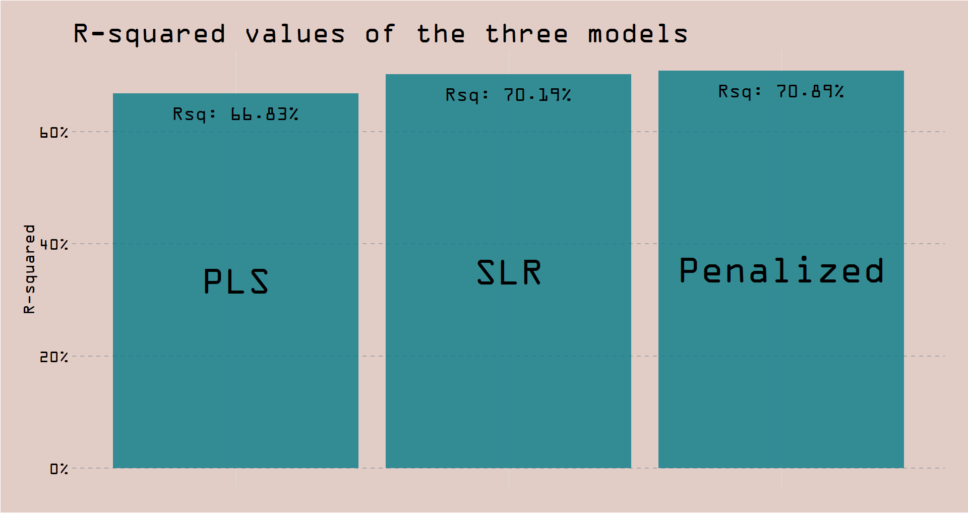
## 1 0.709 PenalizedOkay, we made it! We built 3 models and saved their R-squared. How did they perform? Let’s make some viz!

Evaluation
This plot of R-Squared you’ve seen already at the very beginning. It’s pretty self-explanatory, so I’ll just quickly show you the code.
library(scales)
library(emo)
library(extrafont)
theme_set(theme_light())

rsqs <- slr_rsq %>%
  rbind(pls_rsq) %>%
  rbind(penalized_rsq) %>%
  mutate(model = fct_reorder(model, .estimate))
plot1 <- ggplot(data = rsqs, aes(model, .estimate)) +
geom_col(fill = "#077b88", alpha = 0.8) +
geom_text(aes(model, .estimate / 2, label = model),
family = "OCR A Extended",
size = 20) +
geom_text(aes(model, label = paste("Rsq:", percent(.estimate))),
family = "OCR A Extended",
size = 10,
vjust = 2) +
scale_y_continuous(labels = percent_format()) +
labs(title = "R-squared values of the three models",
y = "R-squared") +
theme(
plot.background = element_rect(fill = "#e2ccc6"),
panel.background = element_rect(fill = "#e2ccc6"),
panel.grid.major.y = element_line(colour = "#a9a9a9", size = 1, linetype = "dashed"),
panel.grid.minor = element_blank(),
panel.border = element_blank(),
axis.ticks = element_blank(),
axis.title.x = element_blank(),
axis.text.x = element_blank(),
axis.title.y = element_text(size = 25, family = "OCR A Extended"),
axis.text.y = element_text(size = 25, family = "OCR A Extended", colour = "black"),
plot.title = element_text(family = "OCR A Extended", size = 43),
plot.margin = unit(c(1.2, 1.2, 1.2, 1.2), "cm")
)
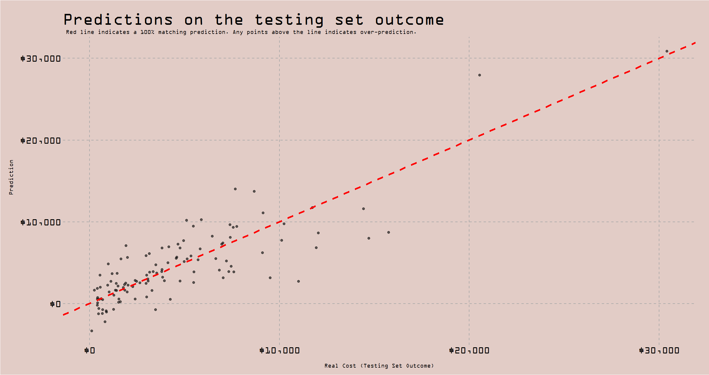
So, the penalized performed best out of the three, although only marginally better than the simple linear regression. Nonetheless, let’s use the penalized model to graph the actual vs predicted plot.
plot2 <- penalized_final %>%
  collect_predictions() %>%
  ggplot(aes(real_cost, .pred)) +
  geom_point(alpha = 0.6, size = 3) +
  geom_abline(color = "red", linetype = "dashed", size = 2) +
  scale_y_continuous(labels = dollar_format()) +
  scale_x_continuous(labels = dollar_format()) +
  labs(title = "Predictions on the testing set outcome",
       subtitle = "Red line indicates a 100% matching prediction. Any points above the line indicates over-prediction.",
       x = "Real Cost (Testing Set Outcome)",
       y = "Prediction") +
  theme(
    plot.background = element_rect(fill = "#e2ccc6"),
    panel.background = element_rect(fill = "#e2ccc6"),

    panel.grid.major.y = element_line(colour = "#a9a9a9", size = 1, linetype = "dashed"),
    panel.grid.major.x = element_line(colour = "#a9a9a9", size = 1, linetype = "dashed"),

    panel.grid.minor = element_blank(),
    panel.border = element_blank(),

    axis.ticks = element_blank(),
    axis.title.x = element_text(size = 15, family = "OCR A Extended", vjust = -5),
    axis.text.x = element_text(size = 25, family = "OCR A Extended", colour = "black"),
    axis.title.y = element_text(size = 15, family = "OCR A Extended", vjust = 5, hjust = 0.55),
    axis.text.y = element_text(size = 25, family = "OCR A Extended", colour = "black"),

    plot.title = element_text(family = "OCR A Extended", size = 43),
    plot.subtitle = element_text(family = "OCR A Extended", size = 15, hjust = 0.01),
    plot.margin = unit(c(1.2, 1.2, 1.2, 1.2), "cm")
  )
This plot visualizes if the model exhibits any patterns, for a particular range of the correct “answer”. From what I can tell, there isn’t anything egregiously eye-catching, I’ll even point out that the one observation around $30,000 seems to have been well-predicted.
That’s it! To recap, we used the tidymodels family to build 3 different linear regression models, compared their performance using R-squared. The best model we picked the penalized model, with its hyperparameters tuned to be of minimal ridge penalty.
See you next time!